Nature’s voice is mathematics, its language is differential equations.

This quote, which I did once find attributed to Galileo, has bounced around scientific circles for quite some time and its sentiment has been shared by many scientists and much research in physics and chemistry has backed it up. Differential equations seem to describe much of the natural world and by using them, our power to model the world expands. While Galileo couldn’t have imagined it, these same mathematical tools now let us generate images, not just model planets. This blog post aims to cover a more recent use case of this tool: flow matching models.

Introduction and Intuition

To start, an analogy. Imagine you are an explorer in the 16th century getting ready to set sail across a vast ocean. You start in Europe and are setting sail to the Americas, hoping for riches. You know what Europe looks like and can start from many different points on the continent. You also have some information on some major landmarks in the Americas from the work of previous explorers. This is where you and I stand as we embark on our flow matching journey. We have some noise that is distributed according to a multivariate standard Gaussian and we can sample from this, just like how we can start our voyage from anywhere in Europe. We also have some pictures, but we don’t know the exact distribution of these images, just like how we know of some landmarks in the Americas but don’t have a great map of the continent.

Now in order to make the journey across the Atlantic, we need to follow a path. For our intrepid voyager, this means following the trade winds across the ocean. For our flow matching model, it means following a path defined by a vector field. Our model will learn this vector field, and we can use ODE solvers to trace this path and generate our output. Similarly, our captain can use a compass and map to follow the trade winds we’ve charted.

Let’s contrast this with another major architecture for training generative models: diffusion. Imagine diffusion as your rival explorer who throws caution to the wind. Instead of studying the trade winds before setting sail, they simply begin their journey and soldier through whatever bumps they encounter along the way. Our diffusion rival accepts the jaggedness of the storm, reacting to every random gust of noise, hoping to eventually stumble upon the shore.

In contrast, our flow matching explorer learns the winds themselves and charts efficient, deterministic paths from any starting point in Europe to any destination in the New World. By learning the vector field that transforms Gaussian noise into real images from our dataset, we can efficiently generate new images from new Gaussian noise.

Preparing for the Journey

A quick note: this section will assume some level of familiarity with differential equations.

Now that we have the intuition down for what flow matching is aiming to do, we can get into the “how” for the process. Before we get into that, I want to clarify the terms we are using here and connect back to the analogy one last time to really hammer it home:

• $x_0$: This is simply a sample of pure noise from a multivariate standard Gaussian, $p_{\text{init}} = \mathcal{N}(0, I)$. In our analogy, this is the point in Europe that we set sail from.
• $x_1$: This is a real image sampled from our dataset ($p_{\text{data}}$). This was the landmark that we knew of in the Americas in our analogy.
• $t$: A value between $0$ and $1$. $t=0$ represents the moment we leave the docks in Europe, and $t=1$ is the moment we arrive at the shore of the Americas. In our generative process, $t=0$ is the time at which our image is pure Gaussian noise, $t=1$ is when our image is a real image from $p_{data}$, and every in between step is some version of the image with less noise.

Now our goal is to model the winds that will blow any ship from that point $x_0$ to the real image $x_1$. This model of the wind is a vector field, $u_t$, and the particular path that we want to follow is called a flow, $\psi_t$.

Before we set sail, let’s stock the ship with the necessary provisions. Just as a navigator needs maps, a compass, and navigational tables, our computational voyage requires its own essential tools:

import math
import os
from dataclasses import dataclass

import torch
import torch.nn as nn
import torch.nn.functional as F
from torch.utils.data import DataLoader
from torchvision import datasets, transforms
from torchvision.utils import save_image, make_grid

Let’s also plan out some of our voyage. It’s always good to be prepared. Here we define some key hyperparameters:

@dataclass
class CFG:
    device: str = "cuda" if torch.cuda.is_available() else "cpu"
    batch_size: int = 256
    lr: float = 2e-4
    epochs: int = 50

    # Flow matching params
    sigma_min: float = 0.1  # small endpoint noise
    t_eps: float = 1e-5      # avoid exact endpoints

    # Sampling params
    sample_steps: int = 150   # RK4 steps from t=0->1
    n_samples: int = 64
    out_dir: str = "fm_out"

cfg = CFG()
os.makedirs(cfg.out_dir, exist_ok=True)
print("Using device:", cfg.device)

The learning rate controls how quickly the navigator updates its internal map of the winds, while the batch size determines how many ships we observe at once. The parameter $\sigma_{\min}$ enforces a small amount of uncertainty at landfall. We are aiming for the general area of our destination instead of trying to land at some impossibly precise point. Finally, the sampling parameters determine how finely we trace the learned route during inference.

A Quick Differential Equations Aside

The solution to an ODE is defined by a trajectory that maps some time $t$ to some location in the space $\mathbb{R}^d$.

Every ODE is defined by some vector field. Going back to the analogy, the vector field is all of the winds that blow across the Atlantic. The solution mentioned above is one such path along one current that can take one ship across the ocean. We write out an ODE defined by a vector field as follows:

The top line says that our ODE is defined according to some vector field $u_t$ with some initial conditions $x_0$. The derivative of $X_t$ is given by the direction of the vector field. In order to find the flow $\psi_t$, we need some initial conditions $X_0 = x_0$ at some $t = 0$. The flow will tell us the current state when we plug in some time $t$. In our analogy, it would allow us to know exactly where the ship is at some time $t$ just by knowing the initial conditions of the ship. This is written out as follows:

\(\psi : \mathbb{R}^d \times [0, 1] \mapsto \mathbb{R}^d, \quad (x_0, t) \mapsto \psi_t(x_0)\) \(\frac{\mathrm{d}}{\mathrm{d}t} \psi_t(x_0) = u_t(\psi_t(x_0))\) \(\psi_0(x_0) = x_0\)

A note on $\sigma_{\min}$.
In practice, flow matching models do not force trajectories to land exactly on a data point at $t=1$. Instead, the endpoint distribution is taken to be a narrow Gaussian centered at $x_1$, with variance $\sigma_{\min}^2 I$. This small but nonzero noise level prevents singular behavior in the vector field, stabilizes training, and improves numerical behavior during ODE sampling. Think of it as aiming for a harbor rather than a single dock. We want to reach the general area, allowing for natural variation in our final approach. In the idealized limit $\sigma_{\min} \to 0$, the target velocity reduces to the intuitive expression $x_1 - x_0$.

Numerical Solvers

In an ideal world, we could write down a formula that tells us exactly where a ship will be at any time $t$ given the wind field $u_t$. Unfortunately, for most vector fields, including the ones our neural networks learn, no such closed-form solution exists. Instead, we must approximate the trajectory by taking small steps forward in time.

Euler’s Method

The Euler method is a first-order numerical method for solving ODEs. Given $\frac{dx(t)}{dt} = f(t, x)$ and $x(t_0) = x_0$, the Euler method solves the problem via an iterative scheme for $i = 0, 1, \ldots, N-1$ such that

where $\alpha$ is the step size.

At each step, we move in the direction the wind is currently blowing, scaled by our step size. Imagine you’re on a ship and you look at your compass (the vector field) to see which direction to sail. You sail in that direction for a small time $\alpha$, then stop and check your compass again.

However, this method has a critical flaw. If the wind is changing direction as we sail, we’ll overshoot or undershoot the true path because we’re using outdated information. The Euler method only achieves first-order accuracy, meaning errors add up fast.

Example: Consider the ODE \(\frac{dx(t)}{dt} = \frac{x(t) + t^2 - 2}{t + 1}.\)

If we apply the Euler method with step size $\alpha$, then the iteration will take the form

In code, this looks like:

# Simple Euler integration
dt = 1.0 / num_steps
for i in range(num_steps):
    t = i * dt
    v = model(x, t)
    x = x + dt * v  # Just move in current direction

Runge-Kutta (RK4) Method

The Runge-Kutta method is another popularly used ODE solver that achieves much higher accuracy. The RK4 update rule is

where the quantities $k_1, k_2, k_3$ and $k_4$ are defined as

RK4 is like having an experienced helmsman who doesn’t just look at the current wind, but tries to guess how it will change over the next interval. At each step, RK4 makes four evaluations:

1. $k_1$: Check the wind at our current position
2. $k_2$: Predict where we’d be at the midpoint if we followed $k_1$, then check the wind there
3. $k_3$: Predict where we’d be at the midpoint if we followed $k_2$, then check the wind there
4. $k_4$: Predict where we’d be at the endpoint if we followed $k_3$, then check the wind there

Then combine these four predictions with the weights shown above: the midpoint evaluations ($k_2$ and $k_3$) are weighted twice as heavily as the endpoint evaluations.

The genius of RK4 is that by sampling the vector field at multiple points within each interval and weighting them appropriately, we achieve fourth-order accuracy. This means that if we halve the step size, our error decreases by a factor of 16, compared to just 2 for Euler’s method.

In our implementation, this looks like:

# RK4 integration - used in our sample() function
dt = 1.0 / cfg.sample_steps
for i in range(cfg.sample_steps):
    t0 = (i + 0.5) * dt
    t = torch.full((x.size(0),), t0, device=x.device)
    
    k1 = model(x, t)
    k2 = model(x + 0.5*dt*k1, torch.clamp(t + 0.5*dt, cfg.t_eps, 1.0 - cfg.t_eps))
    k3 = model(x + 0.5*dt*k2, torch.clamp(t + 0.5*dt, cfg.t_eps, 1.0 - cfg.t_eps))
    k4 = model(x + dt*k3, torch.clamp(t + dt, cfg.t_eps, 1.0 - cfg.t_eps))
    
    x = x + (dt/6.0) * (k1 + 2*k2 + 2*k3 + k4)

Why does this matter for Flow Matching?

Because we learned straight-line OT paths, our vector field is relatively smooth and predictable. This means RK4 can trace these paths very accurately with relatively few steps (50-150 in our implementation), whereas diffusion models with their noisy, curved trajectories often need hundreds of steps even with sophisticated solvers. The smoothness of the learned vector field and the accuracy of the numerical solver work together for efficient, high-quality generation.

Plotting the Probability Path

So far, we have focused on the journey of a single ship. One starting point $x_0$, one destination $x_1$, and one path through the ocean defined by a vector field. But to train a generative model, we must zoom out.

The flow $\psi_t$ describes how one individual point moves over time. The probability path $p_t$, on is the satellite view (I know I said it’s the 16th century but use your imagination). It captures how an entire distribution of ships evolves as time progresses. At $t=0$, this distribution is cloud of ships spread across Europe, sampled from a standard Gaussian. By $t=1$, that cloud has condensed and reshaped itself into the complex structure of real images from our dataset.

Formally, $p_t$ is the marginal distribution induced by transporting noise samples forward in time under the learned vector field. If we could directly compute the true vector field that depicts this, we could train a neural network by minimizing

Here, $v_t^\theta(x)$ is our neural network and $u_t^{\text{target}}(x)$ is the true velocity field that moves the entire distribution $p_t$ through time.

Unfortunately, this global wind map is extraordinarily complex. Modeling it directly would require knowing the full intermediate distributions between Gaussian noise and real images, which is computationally intractable.

The Continuity Equation

Unfortunately this next part will require some physics. The reason we can use a vector field to shape a distribution is due to the Continuity Equation. In our analogy, if we know how the wind is blowing at every coordinate in the Atlantic, we can predict how the entire fleet of ships will spread out or cluster together over time. Mathematically, a probability path $p_t$ is said to be consistent with a vector field $u_t$ if they satisfy the following first-order partial differential equation:

This equation is just saying that probability is conserved across our whole vector field. Ships simply move across from one state to another such as moving from noise to real data.

When we train our model, we are looking for some set of parameters for $v^{\theta}_t$ that will satisfy the continuity equation. The conditional flow matching proof that comes later on shows that we can satisfy this global “conservation of ships” equation by only ever looking at individual, simple paths.

Conditional and Marginal Vector Fields

While our navigator trains by looking at a single ship’s path from $x_0$ to a specific $x_1$, the ocean is actually full of ships heading to different destinations. During training, we define a conditional vector field $u_t(x \mid x_1)$, which is the specific wind needed to reach landmark $x_1$.

However, when we actually set sail with new noise at inference time, we don’t know which landmark we are heading toward. The model must instead follow the marginal vector field, $u_t(x)$. This is the “average” of all possible conditional winds at a specific point in the ocean, weighted by how likely it is that a ship at $x$ is headed to a particular $x_1$:

In simpler terms, if multiple ships heading to different cities all pass through the same patch of sea, the model learns the “consensus” wind that represents the aggregate flow of the entire distribution. In more mathematical terms, the marginal vector field is the aggregation of every conditional vector field where we marginalize the condition out. As we established before, this process is intractable so we cannot learn the marginal vector field in this way.

Score Functions

Before we move forward, I want to connect flow matching back to diffusion, because although this post has repeatedly pitted the two against each other, diffusion can be viewed as a stochastic counterpart to flow matching that uses stochastic differential equations instead of ordinary differential equations.

If you have spent any time in the world of generative modeling, you have likely encountered the score function, denoted as $\nabla \log p_t(x)$. In our analogy, if the vector field $u_t(x)$ is the trade wind, then the score function is the lay of the land. The score function points in the direction where the cloud of ships is most dense, essentially telling you where the data distribution is most concentrated. While it tells you where the landmark is, it doesn’t necessarily dictate the most efficient path to get there. For the Gaussian probability paths we often use, these two concepts are mathematically intertwined; the marginal vector field $u_t(x)$ can be expressed as a combination of a time-dependent drift and the score function.

The primary differentiator between flow matching and diffusion is the efficiency of the journey. Diffusion models follow the score function, which often results in highly curved, jagged, and stochastic trajectories. This is why our “diffusion rival” requires hundreds of steps. They are constantly fighting the noise of the storm and making small corrections to stay on track. In contrast, by using optimal transport (OT) paths, flow matching targets a constant, straight-line velocity: $x_1 - (1 - \sigma_{\min}) x_0$. Because the resulting vector field is “flatter” and deterministic, we don’t need a hundred small corrections. We can simply set our heading and arrive at the shore in a fraction of the time, often in as few as 10 to 20 steps.

Conditional Flow Matching

Now we get back on track with our explorer sailing the seas.

Instead of mapping the entire ocean at once (our intractable integral), flow matching takes a more clever approach. We condition on a specific destination $x_1$ and only consider voyages that end at that point. In other words, rather than learning the marginal probability path $p_t$, we define a conditional probability path $p_t(\cdot \mid x_1)$.

In practice, this conditional path is chosen to be simple. A common and effective choice is a Gaussian whose mean moves toward $x_1$ while its variance shrinks over time. Early in the journey, ships are widely dispersed. As $t$ increases, they become more concentrated around their destination.

For a particular and important case, known as the optimal transport (OT) path, the corresponding flow map takes a particularly elegant form:

This path is linear in time and induces a constant velocity field

When $\sigma_{\min}$ is small, this velocity closely resembles a straight push from noise toward data. In the idealized limit where $\sigma_{\min} \to 0$, it reduces to the intuitive expression $x_1 - x_0$.

This constant velocity becomes the regression target for our neural network. Rather than learning a complex, stochastic process, the model simply learns the steady winds that carry ships from their noisy origins to their destinations. We can implement this sampling process in code:

def sample_ot_path(x1):
    """Sample a point along the optimal transport path.
    
    This function embodies our voyage planning: given a destination (x1),
    we randomly choose when to observe the ship (t), determine where it 
    started (x0), and compute both its current position (xt) and the 
    constant wind that should be blowing (u).
    """
    B = x1.size(0)
    # Choose random observation times, avoiding exact endpoints
    t = torch.rand(B, device=x1.device)
    t = t * (1 - 2 * cfg.t_eps) + cfg.t_eps
    
    # Each ship departs from a random point in Europe (Gaussian noise)
    x0 = torch.randn_like(x1)
    
    # Compute current position along the linear path
    a = 1 - (1 - cfg.sigma_min) * t
    xt = a[:, None, None, None] * x0 + t[:, None, None, None] * x1
    
    # The constant OT wind that should blow at this position
    u = x1 - (1 - cfg.sigma_min) * x0
    
    return t, xt, u

As the model learns thousands of these conditional voyages, each corresponding to a different destination image, it implicitly reconstructs the global probability path. This is the key insight of conditional flow matching: by learning many simple, local maps, we recover the full global transport without ever modeling it directly.

The resulting training objective is

This loss is equivalent to the original flow matching objective up to an additive constant. I have included the proof that shows this because I think it’s a nice proof that can build some understanding but it’s entirely optional for the scope of this paper.

The Navigator’s Code

The allure of flow matching is that the training loop is simple and deterministic.

The first question the navigator must answer is what time it is. The optimal direction to steer depends not only on where the ship is, but also on how far along the voyage it has progressed. Near Europe, the winds behave differently than they do near the Americas.

To make time usable by a neural network, we embed the scalar $t \in [0,1]$ into a higher-dimensional representation using sinusoidal features. In our sailing analogy, it’s like how a chronometer translates the sun’s position into navigational coordinates:

class SinusoidalTimeEmbedding(nn.Module):
    """Encodes time as a rich navigational signal.
    
    Just as a ship's chronometer tells more than just 'morning' or 'evening',
    this embedding transforms scalar time into a high-dimensional representation
    that allows the network to understand subtle temporal nuances.
    """
    def __init__(self, dim):
        super().__init__()
        self.dim = dim

    def forward(self, t):
        # t: (B,) in [0,1]
        half = self.dim // 2
        freqs = torch.exp(
            -math.log(10000) * torch.arange(half, device=t.device).float() / (half - 1)
        )
        args = t[:, None] * freqs[None, :] * 2 * math.pi
        emb = torch.cat([torch.sin(args), torch.cos(args)], dim=-1)
        if self.dim % 2 == 1:
            emb = F.pad(emb, (0, 1))
        return emb

Think of this as giving the ship a sophisticated clock. The same location in the Atlantic can demand different steering depending on whether we just left Europe or we are nearing the Americas. The time embedding turns the scalar $t$ into a more nuanced signal the network can use to adjust its winds.

Time enters the model as a continuous signal rather than a discrete step count. The sinusoidal embedding allows the navigator to smoothly interpolate its behavior across the voyage, much like how seasonal winds change gradually rather than abruptly. This choice ensures that nearby times correspond to nearby representations, which is essential for stable ODE integration.

Next, we construct the navigator itself. This neural network represents the learned vector field $v_\theta(x,t)$. Given the ship’s current position $x$ and the current time $t$, it outputs a velocity vector indicating which direction to move next. Our architecture uses ResBlocks with FiLM (Feature-wise Linear Modulation) conditioning:

class ResBlock(nn.Module):
    """A residual block with time conditioning via FiLM.
    
    FiLM (Feature-wise Linear Modulation) lets time influence how 
    the network processes spatial information.
    """
    def __init__(self, ch, tdim, groups=8):
        super().__init__()
        self.norm1 = nn.GroupNorm(groups, ch)
        self.conv1 = nn.Conv2d(ch, ch, 3, padding=1)
        
        self.norm2 = nn.GroupNorm(groups, ch)
        self.conv2 = nn.Conv2d(ch, ch, 3, padding=1)
        
        # FiLM: time -> (scale, shift)
        self.to_film = nn.Sequential(
            nn.SiLU(),
            nn.Linear(tdim, 2 * ch),
        )
    
    def forward(self, x, t_emb):
        h = self.conv1(F.silu(self.norm1(x)))
        
        # Apply time-dependent modulation
        film = self.to_film(t_emb)[:, :, None, None]
        scale, shift = film.chunk(2, dim=1)
        h = h * (1 + scale) + shift
        
        h = self.conv2(F.silu(self.norm2(h)))
        return x + h

Now we build the complete navigator. We use a U-Net style architecture that processes images while being guided by time. The downsampling and upsampling structure mimics how a navigator zooms out to see the whole ocean, then zooms in for precise local corrections:

class VelocityNet(nn.Module):
    """Our navigator: predicts wind direction v_theta(x,t).
    
    This U-Net processes the current image and time to predict 
    which direction to move next. The architecture mirrors how a 
    navigator considers both broad ocean currents (downsampling) 
    and local conditions (upsampling with skip connections).
    """
    def __init__(self, base=64, tdim=128, groups=8):
        super().__init__()
        self.time = SinusoidalTimeEmbedding(tdim)
        self.time_mlp = nn.Sequential(
            nn.Linear(tdim, tdim),
            nn.SiLU(),
            nn.Linear(tdim, tdim),
        )
        
        self.in_conv = nn.Conv2d(1, base, 3, padding=1)
        
        # Down: observe the broad ocean currents
        self.rb1 = ResBlock(base, tdim, groups)
        self.down = nn.Conv2d(base, base * 2, 4, stride=2, padding=1)
        self.rb2 = ResBlock(base * 2, tdim, groups)
        
        # Mid: deepest understanding of the voyage
        self.mid = ResBlock(base * 2, tdim, groups)
        
        # Up: refine with local corrections
        self.up = nn.ConvTranspose2d(base * 2, base, 4, stride=2, padding=1)
        self.rb3 = ResBlock(base, tdim, groups)
        
        self.out_norm = nn.GroupNorm(groups, base)
        self.out_conv = nn.Conv2d(base, 1, 3, padding=1)
    
    def forward(self, x, t):
        if t.dim() != 1:
            t = t.view(-1)
        
        t_emb = self.time_mlp(self.time(t))
        
        h0 = self.in_conv(x)
        h1 = self.rb1(h0, t_emb)
        
        h2 = self.down(h1)
        h2 = self.rb2(h2, t_emb)
        h2 = self.mid(h2, t_emb)
        
        h3 = self.up(h2)
        h3 = h3 + h1  # skip: recall details from before diving deep
        h3 = self.rb3(h3, t_emb)
        
        out = self.out_conv(F.silu(self.out_norm(h3)))
        return out

During training, we do not simulate entire voyages from start to finish. Instead, we randomly stop ships at intermediate times and ask *what winds should be acting here. Our loss function implements this training objective, with a few practical changes:

def flow_matching_loss(model, x1, beta=0.1, lam=3e-5):
    """Compute the conditional flow matching loss.
    
    We sample random checkpoints along voyages (via sample_ot_path),
    ask our navigator which wind should blow there, and penalize 
    deviations from the true OT wind. The weighting and regularization
    help stabilize trainin.
    """
    t, xt, u = sample_ot_path(x1)
    v = model(xt, t)
    
    # Weight loss by t(1-t): focus more on mid-journey
    w = (t * (1 - t)).view(-1, 1, 1, 1)
    w = w / (w.mean() + 1e-8)
    
    # Smooth L1 is more forgiving of outliers than L2
    per_pixel = F.smooth_l1_loss(v, u, reduction="none", beta=beta)
    return (w * per_pixel).mean() + lam * v.pow(2).mean()

The weighting factor $t(1-t)$ emphasizes the middle of the journey. This makes sense intuitively as at the very start ($t \approx 0$), we’re in pure noise and any direction is fine while near the end ($t \approx 1$), we’re already at the image. The middle is the most crucial part because we are the farthest from our anchors on either end. Learning the middle correctly is what can make or break the model.

To smooth out the navigator’s learning over many voyages, we maintain an Exponential Moving Average (EMA) of the model weights. Think of this as the accumulated wisdom of many expeditions:

class EMA:
    """Exponential Moving Average of model parameters.
    
    Like how charts improve with each expedition's observations,
    EMA maintains a smoothed version of the model that often 
    generalizes better than the latest checkpoint alone.
    """
    def __init__(self, model, decay=0.999):
        self.decay = decay
        self.shadow = {
            k: v.detach().clone()
            for k, v in model.state_dict().items()
        }
    
    @torch.no_grad()
    def update(self, model):
        for k, v in model.state_dict().items():
            self.shadow[k].mul_(self.decay).add_(v.detach(), alpha=1 - self.decay)
    
    def copy_to(self, model):
        model.load_state_dict(self.shadow, strict=True)

The training loop repeatedly sends fleets of ships across random segments of the ocean. Each batch corresponds to many independent voyages, all sharing the same navigator. Over time, the navigator becomes increasingly accurate at predicting which winds will carry ships toward land:

def train():
    """Train the flow matching model on MNIST.
    
    Each epoch represents a season of exploration. Ships depart 
    from random points (noise), head toward different landmarks 
    (digits), and we observe them at random times to learn the 
    prevailing winds.
    """
    transform = transforms.Compose([
        transforms.ToTensor(),
        transforms.Lambda(lambda x: x * 2 - 1)  # Scale to [-1, 1]
    ])
    ds = datasets.MNIST(root=".", train=True, download=True, transform=transform)
    dl = DataLoader(ds, batch_size=cfg.batch_size, shuffle=True)
    
    model = VelocityNet().to(cfg.device)
    opt = torch.optim.AdamW(model.parameters(), lr=cfg.lr)
    
    ema = EMA(model, decay=0.999)
    
    model.train()
    for epoch in range(cfg.epochs):
        for step, (x1, _) in enumerate(dl):
            x1 = x1.to(cfg.device)
            loss = flow_matching_loss(model, x1)
            opt.zero_grad()
            loss.backward()
            opt.step()
            
            ema.update(model)
            
            if step % 200 == 0:
                print(f"Epoch {epoch} Step {step} Loss {loss.item():.4f}")
    
    return model, ema

This loop represents many seasons of exploration. Each batch corresponds to a fleet of ships, each heading toward different destinations and observed at different times. Over repeated epochs, the navigator refines its understanding of the winds until it can reliably guide ships from noise to data across the entire ocean.

Once training is complete, generation is simply navigation. We release new ships from Europe (fresh Gaussian noise) and numerically integrate the learned vector field forward in time. Here we use the Runge-Kutta 4th order (RK4) method:

@torch.no_grad()
def sample(model):
    """Generate images by sailing from noise to data.
    
    Starting from random Gaussian noise (Europa's shores), we follow 
    the learned winds step by step using RK4 integration. Each step 
    asks the navigator for guidance, then combines multiple velocity 
    predictions for a smooth, accurate trajectory.
    """
    x = torch.randn(cfg.n_samples, 1, 28, 28, device=cfg.device)
    dt = 1.0 / cfg.sample_steps
    
    for i in range(cfg.sample_steps):
        # Evaluate at midpoint of interval for stability
        t0 = (i + 0.5) * dt
        t0 = min(max(t0, cfg.t_eps), 1.0 - cfg.t_eps)
        t = torch.full((x.size(0),), t0, device=x.device)
        
        # RK4: four evaluations for a single smooth step
        k1 = model(x, t)
        k2 = model(x + 0.5 * dt * k1, torch.clamp(t + 0.5 * dt, cfg.t_eps, 1.0 - cfg.t_eps))
        k3 = model(x + 0.5 * dt * k2, torch.clamp(t + 0.5 * dt, cfg.t_eps, 1.0 - cfg.t_eps))
        k4 = model(x + dt * k3, torch.clamp(t + dt, cfg.t_eps, 1.0 - cfg.t_eps))
        
        # Weighted combination gives accurate trajectory
        x = x + (dt / 6.0) * (k1 + 2*k2 + 2*k3 + k4)
    
    return (x.clamp(-1, 1) + 1) / 2

The RK4 method evaluates the velocity field at four carefully chosen points within each timestep, then combines them with specific weights. This is analogous to a navigator checking the wind not just at the ship’s current position, but also at anticipated future positions, then steering a course that accounts for all these observations. The result is a much smoother, more accurate trajectory than simple Euler integration.

Viewed end to end, flow matching transforms generative modeling into a problem of learning and following winds. By replacing stochastic correction with deterministic navigation, we gain smoother trajectories, fewer inference steps, and a clearer conceptual link between learning and generation.

Now we can see what the model generates. After training for 50 epochs and using our EMA weights for stability:

model, ema = train()

# Load the smoothed navigator
ema_model = VelocityNet().to(cfg.device)
ema.copy_to(ema_model)
ema_model.eval()

# Set sail from noise
samples = sample(ema_model)
grid = make_grid(samples, nrow=int(math.sqrt(cfg.n_samples)))
save_image(grid, "fm_out/samples.png")

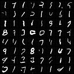
In these results, we can see some numbers but it’s obviously not SOTA or even production grade. However, I’d say that it’s pretty good for what we can get with Colab. There are there definitely some recognizable numbers in there and you can see how with better methods, better data, and better compute, we could definitely get much better results. This implementation serves as a proof of concept—demonstrating that the core Flow Matching principles work exactly as the mathematics predicts.

Why Flow Matching over Diffusion?

You might wonder why we went through the trouble of charting these trade winds when diffusion is already so popular. The benefits come when it is time to actually set sail (inference).

Because we trained our model on straight-line paths, the resulting trajectories are incredibly smooth. In practical terms, this means you can generate high-quality images in far fewer steps. While Diffusion often requires dozens or hundreds of “corrections” to reach the data distribution, Flow Matching can often reach the shore in 10–20 steps using a simple Euler ODE solver or achieve even better quality with 50-150 RK4 steps as we did here.

Next, diffusion is inherently noisy; every time you generate an image, you are at the mercy of the storm. Flow Matching is a Continuous Normalizing Flow. Once you pick your starting point $x_0$, the path to the final image is deterministic. This makes the model easier to debug and allows for smooth interpolation between different images. Want to see a “3” gradually morph into an “8”? Just linearly interpolate the starting noise.

Finally, we have successfully traded complex variance-preserving schedules for a simple line: $x_t = (1-t)x_0 + tx_1$. This simplicity makes Flow Matching much easier to scale to massive datasets and complex architectures. The training objective is straightforward regression, the sampling is deterministic ODE integration, and the entire framework rests on solid mathematical foundations rather than carefully tuned noise schedules.

References

For those who wish to dive deeper into the technical proofs and the broader implications of Flow Matching, I highly recommend the following papers:

• Lipman, Y., Chen, R. T. Q., Ben-Hamu, H., Nickel, M., & Le, M. (2022). Flow matching for generative modeling. arXiv. https://doi.org/10.48550/arXiv.2210.02747

• Holderrieth, P., & Erives, E. (2025). An introduction to flow matching and diffusion models. arXiv. https://doi.org/10.48550/arXiv.2506.02070

• Liu, X., Gong, C., & Liu, Q. (2022). Flow straight and fast: Learning to generate and transfer data with rectified flow. arXiv. https://doi.org/10.48550/arXiv.2209.03003

• Chan, S. H. (2025). Tutorial on diffusion models for imaging and vision. arXiv. https://doi.org/10.48550/arXiv.2403.18103`